10 Gradient Descent Optimisation Algorithms + Cheat Sheet

By Raimi Bin Karim, AI Singapore

(If you want to jump straight to the cheat sheet section then scroll down to the bottom of the post.)

Gradient descent is an optimisation method for finding the minimum of a function. It is commonly used in deep learning models to update the weights of the neural network through backpropagation.

In this post, I will summarise the common gradient descent optimisation algorithms used in the popular deep learning frameworks (e.g. TensorFlow, Keras, PyTorch, Caffe). The purpose of this post is to make it easy to read and digest (using consistent nomenclature) since there aren’t many such summaries out there, and as a cheat sheet if you want to implement them from scratch.

I have implemented SGD, momentum, Nesterov, RMSprop and Adam in a linear regression problem using gradient descent demo here using JavaScript.

What do gradient descent optimisers do?

 
There are 3 main ways how these optimisers can act upon gradient descent:

     (1) modifying the learning rate component, α, or
     (2) modifying the gradient component, ∂L/∂w, or
     (3) both.

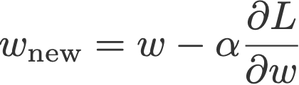
See the last term in Eqn. 1 below:

Learning rate schedulers vs. Gradient descent optimisers
The main difference between these two is that gradient descent optimisers adapt the learning rate component by multiplying the learning rate with a factor that is a function of the gradients, whereas learning rate schedulers multiply the learning rate by a factor which is a constant or a function of the time step.

For (1), these optimisers multiply a positive factor to the learning rate, such that they become smaller (e.g. RMSprop). For (2), optimisers usually make use of the moving averages of the gradient (momentum), instead of just taking one value like in vanilla gradient descent. Optimisers that act on both (3) are like Adam and AMSGrad.

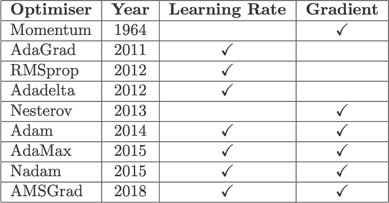
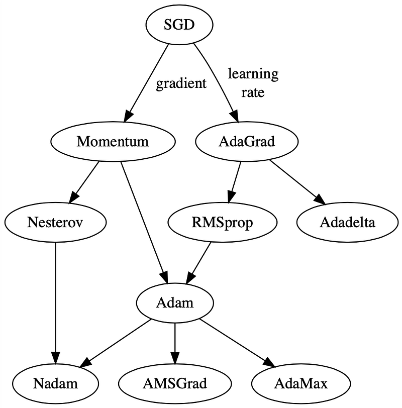
Fig. 3 is an evolutionary map of how these optimisers evolved from the simple vanilla stochastic gradient descent (SGD), down to the variants of Adam. SGD initially branched out into two main types of optimisers: those which act on (i) the learning rate component, through momentum and (ii) the gradient component, through AdaGrad. Down the generation line, we see the birth of Adam (pun intended ????), a combination of momentum and RMSprop, a successor of AdaGrad. You don’t have to agree with me, but this is how I see them ????.

Notations

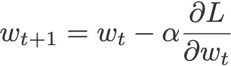
• t — time step
• w — weight/parameter which we want to update
• α — learning rate
• ∂L/∂w — gradient of L, the loss function to minimise, w.r.t. to w
• I have also standardised the notations and Greek letters used in this post (hence might be different from the papers) so that we can explore how optimisers ‘evolve’ as we scroll.

Content

1. Stochastic Gradient Descent
2. Momentum
3. NAG
4. AdaGrad
5. RMSprop
6. Adadelta
7. Adam
8. AdaMax
9. Nadam
10. AMSGrad

1. Stochastic Gradient Descent

 
The vanilla gradient descent updates the current weight w_t  using the current gradient ∂L/∂w_t multiplied by some factor called the learning rate, α.

2. Momentum

 
Instead of depending only on the current gradient to update the weight, gradient descent with momentum (Polyak, 1964) replaces the current gradient with V_t (which stands for velocity), the exponential moving average of current and past gradients (i.e. up to time t). Later in this post, you will see that this momentum update becomes the standard update for the gradient component.

where

and V initialised to 0.

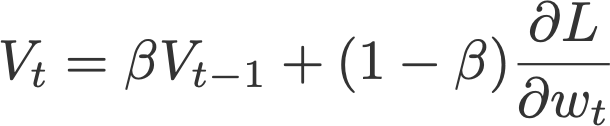
Common default value:

• β = 0.9

Note that many articles reference the momentum method to the publication by Ning Qian, 1999. However, the paper titled Sutskever et al. attributed the classical momentum to a much earlier publication by Polyak in 1964, as cited above. (Thank you to James for pointing this out.)

3. Nesterov Accelerated Gradient (NAG)

 
After Polyak had gained his momentum (pun intended ????), a similar update was implemented using Nesterov Accelerated Gradient (Sutskever et al., 2013). This update utilises V, the exponential moving average of what I would call projected gradients.

where

and V initialised to 0.

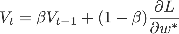
The last term in the second equation is a projected gradient. This value can be obtained by going ‘one step ahead’ using the previous velocity (Eqn. 4). This means that for this time step t, we have to carry out another forward propagation before we can finally execute the backpropagation. Here’s how it goes:

1. Update the current weight w_t to a projected weight w* using the previous velocity.

 
2. Carry out forward propagation, but using this projected weight.
3. Obtain the projected gradient ∂L/∂w*.
4. Compute V_t and w_t+1 accordingly.

Common default value:

• β = 0.9

Note that the original Nesterov Accelerated Gradient paper (Nesterov, 1983) was not about stochastic gradient descent and did not explicitly use the gradient descent equation. Hence, a more appropriate reference is the above-mentioned publication by Sutskever et al. in 2013, which described NAG’s application in stochastic gradient descent. (Again, I’d like to thank James’s comment on Hacker News for pointing this out.)

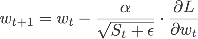
4. AdaGrad

 
Adaptive gradient, or AdaGrad (Duchi et al., 2011), works on the learning rate component by dividing the learning rate by the square root of S, which is the cumulative sum of current and past squared gradients (i.e. up to time t). Note that the gradient component remains unchanged like in SGD.

where

and S initialised to 0.

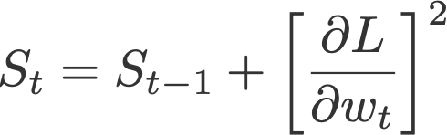
Notice that ε is added to the denominator. Keras calls this the fuzz factor, a small floating point value to ensure that we will never have to come across division by zero.

Default values (from Keras):

• α = 0.01
• ε = 10⁻⁷

5. RMSprop

 
Root mean square prop or RMSprop (Hinton et al., 2012) is another adaptive learning rate that is an improvement of AdaGrad. Instead of taking cumulative sum of squared gradients like in AdaGrad, we take the exponential moving average of these gradients.

where

and S initialised to 0.

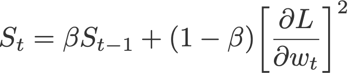
Default values (from Keras):

• α = 0.001
• β = 0.9 (recommended by the authors of the paper)
• ε = 10⁻⁶

6. Adadelta

 
Like RMSprop, Adadelta (Zeiler, 2012) is also another improvement from AdaGrad, focusing on the learning rate component. Adadelta is probably short for ‘adaptive delta’, where delta here refers to the difference between the current weight and the newly updated weight.

The difference between Adadelta and RMSprop is that Adadelta removes the use of the learning rate parameter completely by replacing it with D, the exponential moving average of squared deltas.

where

with D and S initialised to 0, and

Default values (from Keras):

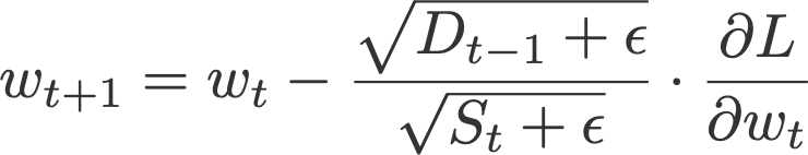
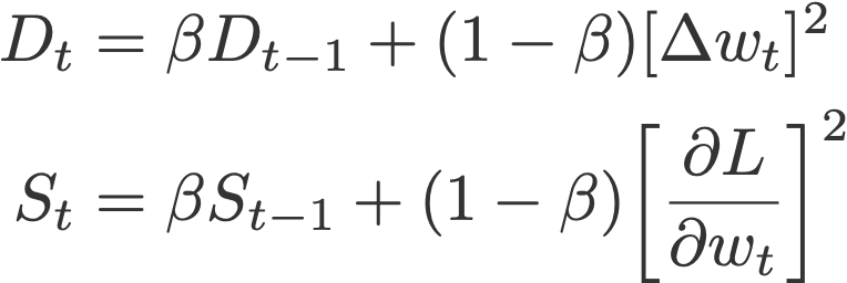
• β = 0.95
• ε = 10⁻⁶

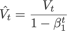
7. Adam

 
Adaptive moment estimation, or Adam (Kingma & Ba, 2014), is a combination of momentum and RMSprop. It acts upon

      (i) the gradient component by using V, the exponential moving average of gradients (like in momentum), and
      (ii) the learning rate component by dividing the learning rate α by square root of S, the exponential moving average of squared gradients (like in RMSprop).

where

are the bias corrections, and

with V and S initialised to 0.

Proposed default values by the authors:

• α = 0.001
• β₁ = 0.9
• β₂ = 0.999
• ε = 10⁻⁸

8. AdaMax

 
AdaMax (Kingma & Ba, 2015) is an adaptation of the Adam optimiser by the same authors using infinity norms (hence ‘max’). V is the exponential moving average of gradients, and S is the exponential moving average of past p-norm of gradients, approximated to the max function as seen below (see paper for convergence proof).

where

is the bias correction for V and

with V and S initialised to 0.

Proposed default values by the authors:

• α = 0.002
• β₁ = 0.9
• β₂ = 0.999

9. Nadam

 
Nadam (Dozat, 2015) is an acronym for Nesterov and Adam optimiser. The Nesterov component, however, is a more efficient modification than its original implementation.

First we’d like to show that the Adam optimiser can also be written as:

Nadam makes use of Nesterov to update the gradient one step ahead by replacing the previous V_hat in the above equation to the current V_hat:

where

and

with V and S initialised to 0.

Default values (taken from Keras):

• α = 0.002
• β₁ = 0.9
• β₂ = 0.999
• ε = 10⁻⁷

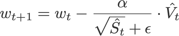
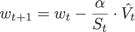
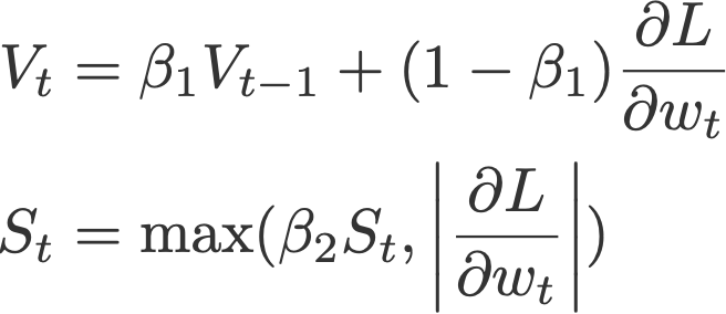
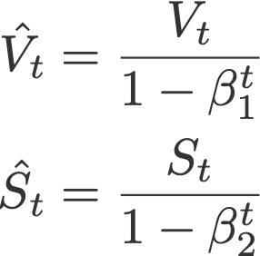
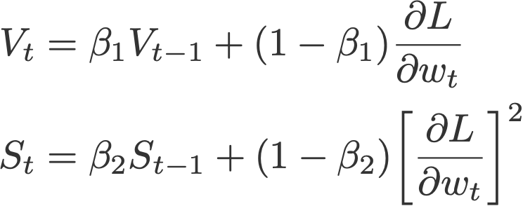
10. AMSGrad

 
Another variant of Adam is the AMSGrad (Reddi et al., 2018). This variant revisits the adaptive learning rate component in Adam and changes it to ensure that the current S is always larger than the previous time step.

where

and

with V and S initialised to 0.

Default values (taken from Keras):

• α = 0.001
• β₁ = 0.9
• β₂ = 0.999
• ε = 10⁻⁷

Intuition

Here, I’d like to share with you some intuition on why gradient descent optimisers use exponential moving average for the gradient component and root mean square for the learning rate component.

Why take exponential moving average of gradients?

We need to update the weight, and to do so we need to make use of some value. The only value we have is the current gradient, so let’s utilise this to update the weight.

But taking only the current gradient value is not enough. We want our updates to be ‘better guided’. So let’s include previous gradients too.

One way to ‘combine’ the current gradient value and information of past gradients is that we could take a simple average of all the past and current gradients. But this means each of these gradients are equally weighted. This would not be intuitive because spatially, if we are approaching the minimum, the most recent gradient values might provide more information that the previous ones.

Hence the safest bet is that we can take the exponential moving average, where recent gradient values are given higher weights (importance) than the previous ones.

Why divide learning rate by root mean square of gradients?

The goal is to adapt the learning rate component. Adapt to what? The gradient. All we need to ensure is that when the gradient is large, we want the update to be small (otherwise, a huge value will be subtracted from the current weight!).

In order to create this effect, let’s divide the learning rate α by the current gradient to get an adapted learning rate.

Bear in mind that the learning rate component must always be positive (because the learning rate component, when multiplied with the gradient component, should have the same sign as the latter). To ensure it’s always positive, we can take its absolute value or its square. Let’s take the square of the current gradient and ‘cancel’ back this square by taking its square root.

But like momentum, taking only the current gradient value is not enough. We want our updates to be ‘better guided’. So let’s make use of previous gradients too. And, as discussed above, we’ll take the exponential moving average of past gradients (‘mean square’), then taking its square root (‘root’), hence ‘root mean square’. All optimisers in this post which act on the learning rate component does this, except for AdaGrad (which takes cumulative sum of squared gradients).

Cheat Sheet

 

Please reach out to me if something is amiss, or if something in this post can be improved! ✌????

References

• An overview of gradient descent optimization algorithms (ruder.io)
• Why Momentum Really Works (distill.pub)

Bio: Raimi Bin Karim is an AI Engineer at AI Singapore

Original. Reposted with permission.

Related:

• Keep it simple! How to understand Gradient Descent algorithm
  
• The Two Phases of Gradient Descent in Deep Learning
  
• How Optimization Works