How to Monitor Machine Learning Models in Real-Time

We present practical methods for near real-time monitoring of machine learning systems which detect system-level or model-level faults and can see when the world changes.

comments

By Ted Dunning, Chief Application Architect, MapR

Introduction

Believe it or not, what you learn in machine learning classes isn’t what you need to know to put machine learning to work. Academic machine learning involves almost exclusively off-line evaluation of machine learning models. This halcyon view is also fostered by the highly publicized contests at Kaggle^[1] or the Netflix challenge^[2]. In the real-world this is, somewhat surprisingly, often only good enough for a rough cut that eliminates the real dogs. For serious production work, online evaluation is often the only option to determine which of several final round candidates might be chosen for further use. As Einstein is rumored to have said, theory and practice are the same, in theory. In practice, they are different. So it is with models. Part of the problem is interaction with other models and systems. Another part has to do with variability of the real world, possibly adversaries at work. It may even literally be sunspots. One particular problem arises when models choose their own training data and thus they exhibit self-reinforcing behavior.

In addition to these difficulties, production models almost always have service level agreements that have to do with how quickly they must produce results and how often they are allowed to fail. These operational considerations can be as important as the accuracy of the model … right results returned late are much worse than mostly right results returned in time.

This article will focus on ways to monitor machine learning systems in real-time or near real-time. Because of this focus, we aren’t going to talk much about getting down to the ground truth of whether a model is producing just the right answer because you often can’t determine that for a long time. For instance, if a fraud model says that an account has been taken over, you may not find out the truth for months. Even so, however, we can often find out if a model is misbehaving (in certain important ways) long before then.

The techniques described here will include the use of coarse functional monitors, non-linear latency histogramming, how to normalize user response data and how to compare score distributions to reference distributions and to canary models. These techniques may sound arcane, but behind the fancy names, each one has a simple heart and doesn’t really require advanced mathematics to understand, implement, or interpret.

It’s a wild world

Let’s talk about what you need to be watching for beyond what you learn in classes. It would absolutely be a simpler world if it worked the way it does in classes and contests, but it isn’t that simple by a long shot. Not only is extracting correct training data a large engineering effort, models running in the wild have to deal with some very complex real-world issues. If you are building a fraud model, the fraudsters will adapt their methods to evade detection by your model. If you are doing marketing, your competitors will always be looking for ways to one-up your efforts. Even with systems that don’t depend on human behavior like airplane engines or factories, surprises still happen. These surprises could be things like a two engine bird strike or like the surprise upgrade of a milling machine or even some contextual issue like market conditions or the weather.

And even if the data environment doesn’t change, there can be equipment failures that cause the world to look strange and surprising.

No matter what kind of machine learning system you are building, you need to monitor your models to make sure that they are still working the way that you think they are. Let’s check out some specific techniques that help spot issues.

Watching the basics

The most basic aspects of model performance is whether it is getting requests and how quickly it is producing results. No model will give good results if you don’t ask for them. And results are no good unless you actually get them in good time.

To monitor whether requests are arriving, you need to record the arrival each incoming request together with the name of the machine where the request has landed and an accurate timestamp. It is typically a bit better to record this data to a persistent stream on a distributed platform because log files can disappear if a machine goes down. It is also better to record request arrival and completion as separate events so that you can distinguish failure to respond from lack of requests. The simplest monitor you can build is to measure the time between requests. One step better is to build a simple predictor of the current request rate based on recent request rates and use the product of the predicted rate times the time since the last request. Even a simple linear model will usually predict request rates an hour ahead of time with less than 10% error which will allow you to raise an alert if requests stop happening. Figure 1 shows an example of how accurately this can work by plotting predicted traffic for the Wikipedia page for “Christmas”.

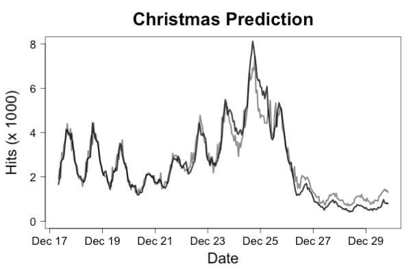
Figure 1. The actual traffic (dark line) versus predicted traffic (gray line) for a traffic prediction model trained on traffic in November. Even though the traffic right around Christmas was radically different from traffic during the training period, predictions were accurate enough to detect system failures very quickly.

The model used for this prediction was a linear regression that used the log of traffic rates for the 4 most recent hours, 24 hours ago and 48 hours ago to predict the log of the traffic now. This prediction can be used to detect request rate anomalies as shown in Figure 2.

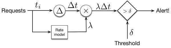
Figure 2. The architecture of a request rate anomaly detector. A threshold is used to determine when the rate drops below the predicted value because the time between events will rise to a high level. The predicted rate is used to normalize this time.

Once we are clear that requests are coming, we can look at whether our model is producing results in a timely manner. To enable this, we need to log the elapsed time as each request is responded to. These log entries should specify a unique ID for the original request, the current time, details of which model and which hardware used to compute the request as well as the elapsed time. As a first cut, we can compute the distribution of the reported elapsed times. For latencies, the best way to do this is by using a non-uniform histogram. We can compute such a histogram for each, say, five minute interval. To monitor performance, we can accumulate a background over a fairly long period of time and plot the recent results against that background distribution. Figure 3 shows what we might see.

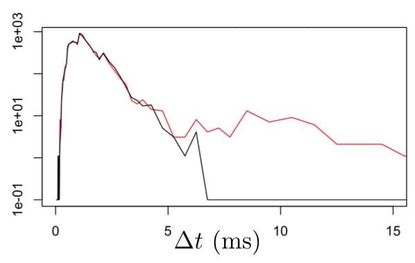
Figure 3. Normal response times in milliseconds (black line) are plotted against response times in which about 1% of responses are substantially delayed. Because of the log-scale on the vertical axis and the non-uniform bin sizes, the change in 99%-ile latency is clearly visible.

These histograms can also be compared using more advanced, automated techniques based on comparing the counts in corresponding bins. One good way to do this is to use a statistical method known as the G-test. Such a test can convert each histogram into a single score that describes how anomalous it is versus the long term background. If the latency measurements that went into a histogram are tagged, then the slow and fast parts of a single histogram can be compared to find out which tags are more common in the slow part. If these tags represent hardware IDs or model versions, then this can be used to target your diagnostic efforts.

But is it RIGHT?!

All of the methods mentioned so far work no matter what the model is supposed to do. But that same generality also means that these techniques can’t tell us anything about the responses that the model is actually producing. Are the results any good? Are they right? We have no real idea. All we know so far is that requests are arriving and results are being produced at historically plausible levels and speeds. Speeds and feeds are nice, but we also need to have some idea when things are not just working, but also whether they are working correctly.

In some kinds of situations, notably when working with marketing models, we can get preliminary feedback about whether our model has done a good job in just a few minutes. In doing this, though, we have to be very careful in comparing different models. In particular, we can’t just compare the number of conversions for each model because as time passes after an ad or offer is presented to a user, more and more conversions will be accrued giving an advantage to older impressions. Figure 4 shows what is going on.

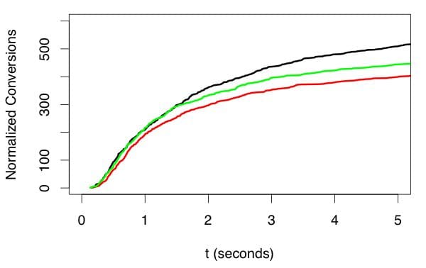
Figure 4. Conversions need to be normalized against the time of the original impression and the number of impressions. Comparisons must also be made at long enough after the impression to get a reliable comparison, but waiting longer than necessary doesn’t help. Here, the green trace seems best at first, but by 2 seconds after impression when only 60% of the conversions have been received, it is clear that black is best and red worst. Picking an appropriate delay allows quickest accurate evaluation of models.

The problem is that each impression of an offer or ad is independent of all others. If the person receiving the impression is going to respond, they will probably respond relatively soon after seeing the impression. Some people will take longer than others, though, and some may respond after a very long time. This means that over time, the conversion rate for any offer will creep up over time. The first thing you have to do, then, is to offset each conversion relative to the time of the corresponding impression. Similarly, some offers will get more impressions than others so you need to scale vertically by the number of impressions, as well.

When you do this, you will see that, because of statistical variation, you have to wait a bit before declaring which offer works best, but you don’t usually have to wait for more than about 60% of the final number responses. This is very important because waiting for 95% of all impressions can take 10x longer than waiting for 50-60% of impressions. This trick is important as well because it allows us to have a near real-time measure of response rate.

Truth may take too long

As nice as real-time ground truth feedback may be, there are lots of use cases where this just isn’t possible. For instance, we may not know even slightly whether a detected fraud is really just that for days or weeks. There are still things that we can do to detect problems quickly, however.

Lots of models produce some sort of score or set of scores. Often these represent some kind of probability estimate. One of the simplest things we can use as a monitor is to look at the score distribution produced by the model. If that distribution changes surprisingly, there is a good chance that there is an important change to the input to the model reflecting some change in the outside world or that the systems that the model depends on, say, for feature extraction have changed in some way. In either case, finding out about the change is the first step in figuring out what is happening.

One of the best ways to detect this kind of change is to use a system known as the t-digest. You can’t really use the logHistogram that we talked about using for latency distributions because scores don’t have the same kind of well understood characteristics as latencies do. The t-digest is a bit more expensive to use, but it can handle pretty much anything that you throw at it. The method, then is to store digests of the score distribution every minute or so tagged with model version and such. To check the score distribution, you can accumulate a number of these stored digests from the past to get the reference distribution and compare this reference to the latest digest.

There are two popular ways to compare distributions. One is to use the deciles of the reference distribution as bin boundaries and then use the latest digest to estimate how many samples are in each bin. If the distributions are the same, then there should be the same number of samples in the recent data in each bin. This can be tested using the G-test as before to get a score that is large when the distributions differ interestingly.

Another approach is to use a value known as a Kolmogorov-Smirnov statistic to detect differences between the reference and recent distributions directly. There is code in the upcoming t-digest release to compute this statistic, but the important factor is that the statistic is large when the distributions differ significantly and smaller when they do not.

Nothing sings like a canary

In general, the more we know about what a model should be doing and the more specific we can be about comparing against reference behavior, the quicker we can reliably detect changes. This is the motivation behind using a canary model. The idea is that we send every request to the current production model as usually, but we also keep an older version of the model around and send every (or nearly every) request to that older version as well. The older model is called a canary.

Because we are sending the exact same requests to both models and because the canary is a model that does nearly the same thing that we want the current model to do, we can compare the output of the two models request by request to get a very specific idea about whether the new model is behaving as expected. The average deviation between canary and the current champion model is a very sensitive indicator of malfunction in the current model, particularly if we choose the canary with an eye to getting a very stable (even if not so incredibly accurate) model.

A canary model is also very handy when we are fielding a potential challenger to our current champion. If we are trying to quantify the risk of rolling out this new challenger to replace our current champion, we can look at the difference between the challenger and the champion as well as the difference between the challenger and the canary. In particular, once we have models that are pretty good and we are making incremental improvements, no new challenger should differ dramatically from the current champion, nor from the canary. Where there is a difference is both where we stand a risk of lower accuracy, but also exactly where the challenger has the opportunity to shine. Focusing in on these specific instances for manual inspection can often give us important insight into whether the challenger is ready to take on the champion.

Wrapping it all up

This article has walked through a range of near real-time monitoring techniques for machine learning models starting with monitors that look purely at the gross operational characteristics of request rate and response times. Those are often very good for detecting systems level problems in evaluating requests. From there, we talked about how to normalize responses for cases like search results or marketing impressions so that they can be compared cleanly and accuracy can be estimated in near real time. For cases where we don’t know exactly what our model should output, we talked about methods for looking for changes in score distributions by comparing to the past performance of the model or by comparing to a canary model.

You probably won’t need to implement all of these methods for monitoring your models, but you should probably implement several of them. You never know what is hiding out there until you look, and you definitely need to know.

^[1] See https://www.kaggle.com/c/GiveMeSomeCredit

^[2] See https://en.wikipedia.org/wiki/Netflix_Prize

Bio: Ted Dunning is Chief Application Architect at MapR and a member of the board of directors for the Apache Software Foundation. He has a long history in building successful startups where machine learning made a big difference in the value of the company. He is listed as inventor on dozens of patents and continues to develop new algorithms and architectures.

Resources:

Related: