Basic Image Data Analysis Using Python – Part 3
Accessing the internal component of digital images using Python packages becomes more convenient to help understand its properties, as well as nature.

Previously we’ve seen some of the very basic image analysis operations in Python. In this last part of basic image analysis, we’ll go through some of the following contents.
Following contents is the reflection of my completed academic image processing course in the previous term. So, I am not planning on putting anything into production sphere. Instead, the aim of this article is to try and realize the fundamentals of a few basic image processing techniques. For this reason, I am going to stick to using SciKit-Image - numpy mainly to perform most of the manipulations, although I will use other libraries now and then rather than using most wanted tools like OpenCV :
I wanted to complete this series into two section but due to fascinating contents and its various outcome, I have to split it into too many part. However, one may find whole series into two section only on my homepage, included below.
Find the whole series: Part 1, Part 2
All source code: GitHub-Image-Processing-Python
But if you’re not interested to redirect, stick with me here . In the previous article, we’ve gone through some of the following basic operations. To keep pace with today’s content, continuous reading is highly appreciated.
- Importing images and observe it’s properties
- Splitting the layers
- Greyscale
- Using Logical Operator on pixel values
- Masking using Logical Operator
I’m so excited, let’s begin!
Intensity Transformation
Let’s begin with importing an image.
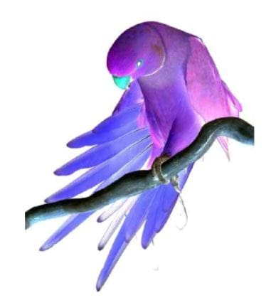
%matplotlibinline

import imageio
import matplotlib.pyplot as plt
import warnings
import matplotlib.cbook
warnings.filterwarnings("ignore",category=matplotlib.cbook.mplDeprecation)

pic=imageio.imread('img/parrot.jpg')

plt.figure(figsize=(6,6))
plt.imshow(pic);
plt.axis('off');

Image Negative
The intensity transformation function mathematically defined as:
S = T(r)
where r is the pixels of the input image and s is the pixels of the output image. T is a transformation function that maps each value of r to each value of s.
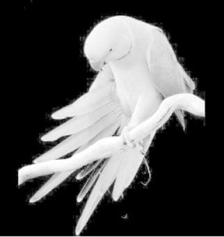
Negative transformation, which is the invert of identity transformation. In negative transformation, each value of the input image is subtracted from the L−1 and mapped onto the output image.
In this case, the following transition has been done:
s=(L–1)–r
So, each value is subtracted by 255. So what happens is that the lighter pixels become dark and the darker picture becomes light. And it results in image negative.
negative =255- pic # neg = (L-1) - img

plt.figure(figsize= (6,6))
plt.imshow(negative);
plt.axis('off');
Log transformation
The log transformations can be defined by this formula:
s=c∗log(r+1)
Where s and r are the pixel values of the output and the input image and c is a constant. The value 1 is added to each of the pixel value of the input image because if there is a pixel intensity of 0 in the image, then log(0) is equal to infinity. So, 1 is added, to make the minimum value at least 1.
During log transformation, the dark pixels in an image are expanded as compared to the higher pixel values. The higher pixel values are kind of compressed in log transformation. This result in the following image enhancement.
The value of c in the log transform adjust the kind of enhancement we are looking for.
%matplotlibinline

import imageio
import numpyasnp
import matplotlib.pyplotasplt

pic=imageio.imread('img/parrot.jpg')
gray=lambda rgb : np.dot(rgb[...,:3],[0.299,0.587,0.114])
gray=gray(pic)


'''
log transform
-> s = c*log(1+r)

So, we calculate constant c to estimate s
-> c = (L-1)/log(1+|I_max|)

'''


max_=np.max(gray)

def log_transform():
return(255/np.log(1+max_))*np.log(1+gray)

plt.figure(figsize=(5,5))
plt.imshow(log_transform(),cmap=plt.get_cmap(name='gray'))
plt.axis('off');
Gamma Correction
Gamma correction, or often simply gamma, is a nonlinear operation used to encode and decode luminance or tristimulus values in video or still image systems. Gamma correction is also known as the Power Law Transform. First, our image pixel intensities must be scaled from the range 0, 255 to 0, 1.0. From there, we obtain our output gamma corrected image by applying the following equation:
Vo = V^(1/G)
Where Vi is our input image and G is our gamma value. The output image, Vo is then scaled back to the range 0-255.
A gamma value, G < 1 is sometimes called an encoding gamma, and the process of encoding with this compressive power-law nonlinearity is called gamma compression; Gamma values < 1 will shift the image towards the darker end of the spectrum.
Conversely, a gamma value G > 1 is called a decoding gamma and the application of the expansive power-law nonlinearity is called gamma expansion. Gamma values > 1 will make the image appear lighter. A gamma value of G = 1 will have no effect on the input image:
import imageio
import matplotlib.pyplotasplt

# Gamma encoding
pic=image io.imread('img/parrot.jpg')
gamma=2.2# Gamma < 1 ~ Dark ; Gamma > 1 ~ Bright

gamma_correction=((pic/255)**(1/gamma))
plt.figure(figsize=(5,5))
plt.imshow(gamma_correction)
plt.axis('off');
The Reason for Gamma Correction
The reason we apply gamma correction is that our eyes perceive color and luminance differently than the sensors in a digital camera. When a sensor on a digital camera picks up twice the amount of photons, the signal is doubled. However, our eyes do not work like this. Instead, our eyes perceive double the amount of light as only a fraction brighter. Thus, while a digital camera has a linear relationship between brightness our eyes have a non-linear relationship. In order to account for this relationship, we apply gamma correction.
There is some other linear transformation function. Listed below:
- Contrast Stretching
- Intensity-Level Slicing
- Bit-Plane Slicing
Convolution
We’ve discussed briefly in our previous article is that, when a computer sees an image, it sees an array of pixel values. Now, depending on the resolution and size of the image, it will see a 32 x 32 x 3 array of numbers where the 3 refers to RGB values or channels. Just to drive home the point, let’s say we have a color image in PNG form and its size is 480 x 480. The representative array will be 480 x 480 x 3. Each of these numbers is given a value from 0 to 255 which describes the pixel intensity at that point.
Like we mentioned before, the input is a 32 x 32 x 3 array of pixel values. Now, the best way to explain a convolution is to imagine a flashlight that is shining over the top left of the image. Let’s say that the flashlight shines cover a 3 x 3 area. And now, let’s imagine this flashlight sliding across all the areas of the input image. In machine learning terms, this flashlight is called a filter or kernel or sometimes referred to as weights or mask and the region that it is shining over is called the receptive field.
Now, this filter is also an array of numbers where the numbers are called weights or parameters. A very important note is that the depth of this filter has to be the same as the depth of the input, so the dimensions of this filter are 3 x 3 x 3.
An image kernel or filter is a small matrix used to apply effects like the ones we might find in Photoshop or Gimp, such as blurring, sharpening, outlining or embossing. They’re also used in machine learning for feature extraction, a technique for determining the most important portions of an image. For more, have a look at Gimp’s excellent documentation on using Image kernel’s. We can find a list of most common kernels here.
Now, let’s take the filter to the top left corner. As the filter is sliding, or convolving, around the input image, it is multiplying the values in the filter with the original pixel values of the image (aka computing element-wise multiplications). These multiplications are all summed up. So now we have a single number. Remember, this number is just representative of when the filter is at the top left of the image. Now, we repeat this process for every location on the input volume. Next step would be moving the filter to the right by a stride or step 1 unit, then right again by stride 1, and so on. Every unique location on the input volume produces a number. We can also choose stride or the step size 2 or more, but we have to care whether it will fit or not on the input image.
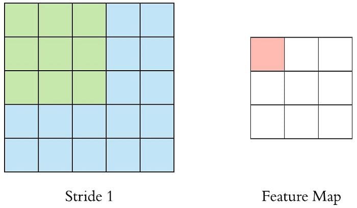
After sliding the filter over all the locations, we will find out that, what we’re left with is a 30 x 30 x 1 array of numbers, which we call an activation map or feature map. The reason we get a 30 x 30 array is that there are 900 different locations that a 3 x 3 filter can fit on a 32 x 32 input image. These 900 numbers are mapped to a 30 x 30 array. We can calculate the convolved image by following:
Convolved: (N−F)/S+1
where N and F represent Input image size and kernel size respectively and S represent stride or step size. So, in this case, the output would be
32−31+1=30
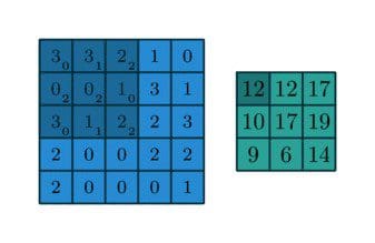
Let’s say we’ve got a following 3x3 filter, convolving on a 5x5 matrix and according to the equation we should get a 3x3 matrix, technically called activation map or feature map.
Let’s take a look somewhat visually,
Moreover, we practically use more filters instead of one. Then our output volume would be 28x28xn (where n is the number of activation map).
By using more filters, we are able to preserve the spatial dimensions better.
However, For the pixels on the border of the image matrix, some elements of the kernel might stand out of the image matrix and therefore does not have any corresponding element from the image matrix. In this case, we can eliminate the convolution operation for these positions which end up an output matrix smaller than the input or we can apply padding to the input matrix.
Now, I do realize that some of these topics are quite complex and could be made in whole posts by themselves. In an effort to remain concise yet retain comprehensiveness, I will provide links to resources where the topic is explained in more detail.
Let’s first apply some custom uniform window to the image. This has the effect of burning the image, by averaging each pixel with those nearby:
%%time
import numpy as np
import imageio
import matplotlib.pyplot as plt
from scipy.signal import convolve2d

def Convolution(image, kernel):
conv_bucket= []
for d in range(image.ndim):
conv_channel= convolve2d(image[:,:,d], kernel,
                               mode="same", boundary="symm")
conv_bucket.append(conv_channel)
returnnp.stack(conv_bucket, axis=2).astype("uint8")


kernel_sizes= [9,15,30,60]
fig, axs=plt.subplots(nrows=1, ncols=len(kernel_sizes), figsize=(15,15));

pic =imageio.imread('img:/parrot.jpg')

for k, ax in zip(kernel_sizes, axs):
    kernel =np.ones((k,k))
    kernel /=np.sum(kernel)
ax.imshow(Convolution(pic, kernel));
ax.set_title("Convolved By Kernel: {}".format(k));
ax.set_axis_off();
Wall time: 43.5 s
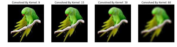
Please, check this more here. I’ve discussed more in depth and played with various types of kernel and showed the differences.
Bio: Mohammed Innat is currently a fourth year undergraduate student majoring in electronics and communication. He is passionate about applying his knowledge of machine learning and data science to areas in healthcare and crime forecast where better solutions can be engineered in the medical sector and security department.
Related: