Multi-Class Text Classification with Scikit-Learn

comments

By Susan Li, Sr. Data Scientist

There are lots of applications of text classification in the commercial world. For example, news stories are typically organized by topics; content or products are often tagged by categories; users can be classified into cohorts based on how they talk about a product or brand online...

However, the vast majority of text classification articles and tutorials on the internet are binary text classification such as email spam filtering (spam vs. ham), sentiment analysis (positive vs. negative). In most cases, our real world problem are much more complicated than that. Therefore, this is what we are going to do today: Classifying Consumer Finance Complaints into 12 pre-defined classes. The data can be downloaded from data.gov.

We use Python and Jupyter Notebook to develop our system, relying on Scikit-Learn for the machine learning components. If you would like to see an implementation in PySpark, read the next article.

Problem Formulation

 
The problem is supervised text classification problem, and our goal is to investigate which supervised machine learning methods are best suited to solve it.

Given a new complaint comes in, we want to assign it to one of 12 categories. The classifier makes the assumption that each new complaint is assigned to one and only one category. This is multi-class text classification problem. I can’t wait to see what we can achieve!

Data Exploration

 
Before diving into training machine learning models, we should look at some examples first and the number of complaints in each class:

import pandas as pd
df = pd.read_csv('Consumer_Complaints.csv')
df.head()

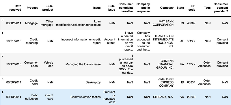
Figure 1

For this project, we need only two columns — “Product” and “Consumer complaint narrative”.

Input: Consumer_complaint_narrative

Example: “I have outdated information on my credit report that I have previously disputed that has yet to be removed this information is more then seven years old and does not meet credit reporting requirements”

Output: product

Example: Credit reporting

We will remove missing values in “Consumer complaints narrative” column, and add a column encoding the product as an integer because categorical variables are often better represented by integers than strings.
We also create a couple of dictionaries for future use.

After cleaning up, this is the first five rows of the data we will be working on:

from io import StringIO

col = ['Product', 'Consumer complaint narrative']
df = df[col]
df = df[pd.notnull(df['Consumer complaint narrative'])]

df.columns = ['Product', 'Consumer_complaint_narrative']

df['category_id'] = df['Product'].factorize()[0]
category_id_df = df[['Product', 'category_id']].drop_duplicates().sort_values('category_id')
category_to_id = dict(category_id_df.values)
id_to_category = dict(category_id_df[['category_id', 'Product']].values)
df.head()

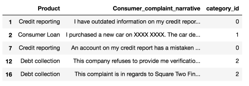
Figure 2

Imbalanced Classes

 
We see that the number of complaints per product is imbalanced. Consumers’ complaints are more biased towards Debt collection, Credit reporting and Mortgage.

import matplotlib.pyplot as plt
fig = plt.figure(figsize=(8,6))
df.groupby('Product').Consumer_complaint_narrative.count().plot.bar(ylim=0)
plt.show()

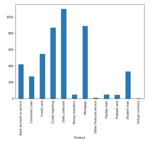
Figure 3

When we encounter such problems, we are bound to have difficulties solving them with standard algorithms. Conventional algorithms are often biased towards the majority class, not taking the data distribution into consideration.In the worst case, minority classes are treated as outliers and ignored. For some cases, such as fraud detection or cancer prediction, we would need to carefully configure our model or artificially balance the dataset, for example by undersampling or oversampling each class.

However, in our case of learning imbalanced data, the majority classes might be of our great interest. It is desirable to have a classifier that gives high prediction accuracy over the majority class, while maintaining reasonable accuracy for the minority classes. Therefore, we will leave it as it is.

Text Representation

 
The classifiers and learning algorithms can not directly process the text documents in their original form, as most of them expect numerical feature vectors with a fixed size rather than the raw text documents with variable length. Therefore, during the preprocessing step, the texts are converted to a more manageable representation.

One common approach for extracting features from text is to use the bag of words model: a model where for each document, a complaint narrative in our case, the presence (and often the frequency) of words is taken into consideration, but the order in which they occur is ignored.

Specifically, for each term in our dataset, we will calculate a measure called Term Frequency, Inverse Document Frequency, abbreviated to tf-idf. We will use sklearn.feature_extraction.text.TfidfVectorizer to calculate a tf-idf vector for each of consumer complaint narratives:

• sublinear_df is set to True to use a logarithmic form for frequency.
• min_df is the minimum numbers of documents a word must be present in to be kept.
• norm is set to l2, to ensure all our feature vectors have a euclidian norm of 1.
• ngram_range is set to (1, 2) to indicate that we want to consider both unigrams and bigrams.
• stop_words is set to "english" to remove all common pronouns ("a", "the", ...) to reduce the number of noisy features.

from sklearn.feature_extraction.text import TfidfVectorizer

tfidf = TfidfVectorizer(sublinear_tf=True, min_df=5, norm='l2', encoding='latin-1', ngram_range=(1, 2), stop_words='english')

features = tfidf.fit_transform(df.Consumer_complaint_narrative).toarray()
labels = df.category_id
features.shape

(4569, 12633)

Now, each of 4569 consumer complaint narratives is represented by 12633 features, representing the tf-idf score for different unigrams and bigrams.

We can use sklearn.feature_selection.chi2 to find the terms that are the most correlated with each of the products:

from sklearn.feature_selection import chi2
import numpy as np

N = 2
for Product, category_id in sorted(category_to_id.items()):
  features_chi2 = chi2(features, labels == category_id)
  indices = np.argsort(features_chi2[0])
  feature_names = np.array(tfidf.get_feature_names())[indices]
  unigrams = [v for v in feature_names if len(v.split(' ')) == 1]
  bigrams = [v for v in feature_names if len(v.split(' ')) == 2]
  print("# '{}':".format(Product))
  print("  . Most correlated unigrams:\n. {}".format('\n. '.join(unigrams[-N:])))
  print("  . Most correlated bigrams:\n. {}".format('\n. '.join(bigrams[-N:])))

# ‘Bank account or service’:

Most correlated unigrams:

• bank
• overdraft

Most correlated bigrams:

• overdraft fees
• checking account

# ‘Consumer Loan’:

Most correlated unigrams:

• car
• vehicle

Most correlated bigrams:

• vehicle xxxx
• toyota financial

# ‘Credit card’:

Most correlated unigrams:

• citi
• card

Most correlated bigrams:

• annual fee
• credit card

# ‘Credit reporting’:

Most correlated unigrams:

• experian
• equifax

Most correlated bigrams:

• trans union
• credit report

# ‘Debt collection’:

Most correlated unigrams:

• collection
• debt

Most correlated bigrams:

• collect debt
• collection agency

# ‘Money transfers’:

Most correlated unigrams:

• wu
• paypal

Most correlated bigrams:

• western union
• money transfer

# ‘Mortgage’:

Most correlated unigrams:

• modification
• mortgage

Most correlated bigrams:

• mortgage company
• loan modification

# ‘Other financial service’:

Most correlated unigrams:

• dental
• passport

Most correlated bigrams:

• help pay
• stated pay

# ‘Payday loan’:

Most correlated unigrams:

• borrowed
• payday

Most correlated bigrams:

• big picture
• payday loan

# ‘Prepaid card’:

Most correlated unigrams:

• serve
• prepaid

Most correlated bigrams:

• access money
• prepaid card

# ‘Student loan’:

Most correlated unigrams:

• student
• navient

Most correlated bigrams:

• student loans
• student loan

# ‘Virtual currency’:

Most correlated unigrams:

• handles
• https

Most correlated bigrams:

• xxxx provider
• money want

They all make sense, don’t you think so?

 
Multi-Class Classifier: Features and Design

• To train supervised classifiers, we first transformed the “Consumer complaint narrative” into a vector of numbers. We explored vector representations such as TF-IDF weighted vectors.
• After having this vector representations of the text we can train supervised classifiers to train unseen “Consumer complaint narrative” and predict the “product” on which they fall.

After all the above data transformation, now that we have all the features and labels, it is time to train the classifiers. There are a number of algorithms we can use for this type of problem.

Naive Bayes Classifier: the one most suitable for word counts is the multinomial variant:

from sklearn.model_selection import train_test_split
from sklearn.feature_extraction.text import CountVectorizer
from sklearn.feature_extraction.text import TfidfTransformer
from sklearn.naive_bayes import MultinomialNB

X_train, X_test, y_train, y_test = train_test_split(df['Consumer_complaint_narrative'], df['Product'], random_state = 0)
count_vect = CountVectorizer()
X_train_counts = count_vect.fit_transform(X_train)
tfidf_transformer = TfidfTransformer()
X_train_tfidf = tfidf_transformer.fit_transform(X_train_counts)

clf = MultinomialNB().fit(X_train_tfidf, y_train)

After fitting the training set, let’s make some predictions.

print(clf.predict(count_vect.transform(["This company refuses to provide me verification and validation of debt per my right under the FDCPA. I do not believe this debt is mine."])))

[‘Debt collection’]

df[df['Consumer_complaint_narrative'] == "This company refuses to provide me verification and validation of debt per my right under the FDCPA. I do not believe this debt is mine."]

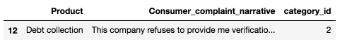
Figure 4

print(clf.predict(count_vect.transform(["I am disputing the inaccurate information the Chex-Systems has on my credit report. I initially submitted a police report on XXXX/XXXX/16 and Chex Systems only deleted the items that I mentioned in the letter and not all the items that were actually listed on the police report. In other words they wanted me to say word for word to them what items were fraudulent. The total disregard of the police report and what accounts that it states that are fraudulent. If they just had paid a little closer attention to the police report I would not been in this position now and they would n't have to research once again. I would like the reported information to be removed : XXXX XXXX XXXX"])))

[‘Credit reporting’]

df[df['Consumer_complaint_narrative'] == "I am disputing the inaccurate information the Chex-Systems has on my credit report. I initially submitted a police report on XXXX/XXXX/16 and Chex Systems only deleted the items that I mentioned in the letter and not all the items that were actually listed on the police report. In other words they wanted me to say word for word to them what items were fraudulent. The total disregard of the police report and what accounts that it states that are fraudulent. If they just had paid a little closer attention to the police report I would not been in this position now and they would n't have to research once again. I would like the reported information to be removed : XXXX XXXX XXXX"]

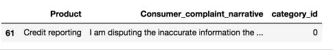
Figure 5

Not too shabby!

Model Selection

 
We are now ready to experiment with different machine learning models, evaluate their accuracy and find the source of any potential issues.

We will benchmark the following four models:

• Logistic Regression
• (Multinomial) Naive Bayes
• Linear Support Vector Machine
• Random Forest

from sklearn.linear_model import LogisticRegression
from sklearn.ensemble import RandomForestClassifier
from sklearn.svm import LinearSVC
from sklearn.model_selection import cross_val_score

models = [
    RandomForestClassifier(n_estimators=200, max_depth=3, random_state=0),
    LinearSVC(),
    MultinomialNB(),
    LogisticRegression(random_state=0),
]
CV = 5
cv_df = pd.DataFrame(index=range(CV * len(models)))
entries = []
for model in models:
  model_name = model.__class__.__name__
  accuracies = cross_val_score(model, features, labels, scoring='accuracy', cv=CV)
  for fold_idx, accuracy in enumerate(accuracies):
    entries.append((model_name, fold_idx, accuracy))
cv_df = pd.DataFrame(entries, columns=['model_name', 'fold_idx', 'accuracy'])

import seaborn as sns

sns.boxplot(x='model_name', y='accuracy', data=cv_df)
sns.stripplot(x='model_name', y='accuracy', data=cv_df, 
              size=8, jitter=True, edgecolor="gray", linewidth=2)
plt.show()

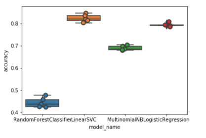
Figure 6

cv_df.groupby('model_name').accuracy.mean()

model_name
LinearSVC: 0.822890
LogisticRegression: 0.792927
MultinomialNB: 0.688519
RandomForestClassifier: 0.443826
Name: accuracy, dtype: float64

LinearSVC and Logistic Regression perform better than the other two classifiers, with LinearSVC having a slight advantage with a median accuracy of around 82%.

Model Evaluation

 
Continue with our best model (LinearSVC), we are going to look at the confusion matrix, and show the discrepancies between predicted and actual labels.

model = LinearSVC()

X_train, X_test, y_train, y_test, indices_train, indices_test = train_test_split(features, labels, df.index, test_size=0.33, random_state=0)
model.fit(X_train, y_train)
y_pred = model.predict(X_test)

from sklearn.metrics import confusion_matrix

conf_mat = confusion_matrix(y_test, y_pred)
fig, ax = plt.subplots(figsize=(10,10))
sns.heatmap(conf_mat, annot=True, fmt='d',
            xticklabels=category_id_df.Product.values, yticklabels=category_id_df.Product.values)
plt.ylabel('Actual')
plt.xlabel('Predicted')
plt.show()

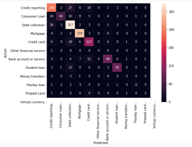
Figure 7

The vast majority of the predictions end up on the diagonal (predicted label = actual label), where we want them to be. However, there are a number of misclassifications, and it might be interesting to see what those are caused by:

from IPython.display import display

for predicted in category_id_df.category_id:
  for actual in category_id_df.category_id:
    if predicted != actual and conf_mat[actual, predicted] >= 10:
      print("'{}' predicted as '{}' : {} examples.".format(id_to_category[actual], id_to_category[predicted], conf_mat[actual, predicted]))
      display(df.loc[indices_test[(y_test == actual) & (y_pred == predicted)]][['Product', 'Consumer_complaint_narrative']])
      print('')

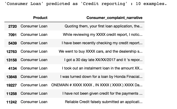
Figure 8

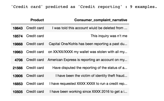
Figure 9

As you can see, some of the misclassified complaints are complaints that touch on more than one subjects (for example, complaints involving both credit card and credit report). This sort of errors will always happen.

Again, we use the chi-squared test to find the terms that are the most correlated with each of the categories:

model.fit(features, labels)

N = 2
for Product, category_id in sorted(category_to_id.items()):
  indices = np.argsort(model.coef_[category_id])
  feature_names = np.array(tfidf.get_feature_names())[indices]
  unigrams = [v for v in reversed(feature_names) if len(v.split(' ')) == 1][:N]
  bigrams = [v for v in reversed(feature_names) if len(v.split(' ')) == 2][:N]
  print("# '{}':".format(Product))
  print("  . Top unigrams:\n       . {}".format('\n       . '.join(unigrams)))
  print("  . Top bigrams:\n       . {}".format('\n       . '.join(bigrams)))

# ‘Bank account or service’:

Top unigrams:

• bank
• account

Top bigrams:

• debit card
• overdraft fees

# ‘Consumer Loan’:

Top unigrams:

• vehicle
• car

Top bigrams:

• personal loan
• history xxxx

# ‘Credit card’:

Top unigrams:

• card
• discover

Top bigrams:

• credit card
• discover card

# ‘Credit reporting’:

Top unigrams:

• equifax
• transunion

Top bigrams:

• xxxx account
• trans union

# ‘Debt collection’:

Top unigrams:

• debt
• collection

Top bigrams:

• account credit
• time provided

# ‘Money transfers’:

Top unigrams:

• paypal
• transfer

Top bigrams:

• money transfer
• send money

# ‘Mortgage’:

Top unigrams:

• mortgage
• escrow

Top bigrams:

• loan modification
• mortgage company

# ‘Other financial service’:

Top unigrams:

• passport
• dental

Top bigrams:

• stated pay
• help pay

# ‘Payday loan’:

Top unigrams:

• payday
• loan

Top bigrams:

• payday loan
• pay day

# ‘Prepaid card’:

Top unigrams:

• prepaid
• serve

Top bigrams:

• prepaid card
• use card

# ‘Student loan’:

Top unigrams:

• navient
• loans

Top bigrams:

• student loan
• sallie mae

# ‘Virtual currency’:

Top unigrams:

• https
• tx

Top bigrams:

• money want
• xxxx provider

They are consistent within our expectation.

Finally, we print out the classification report for each class:

from sklearn import metrics
print(metrics.classification_report(y_test, y_pred, target_names=df['Product'].unique()))

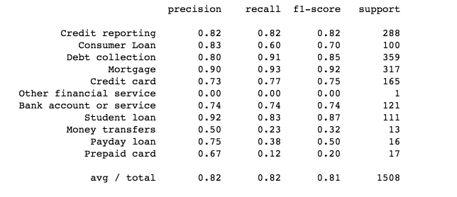
Figure 9

Source code can be found on Github. I look forward to hear any feedback or questions.

 
Bio: Susan Li is changing the world, one article at a time. She is a Sr. Data Scientist, located in Toronto, Canada.

Original. Reposted with permission.

Related:

• Text Classification & Embeddings Visualization Using LSTMs, CNNs, and Pre-trained Word Vectors
• WTF is TF-IDF?
• Natural Language Processing Nuggets: Getting Started with NLP