Receiver Operating Characteristic Curves Demystified (in Python)

comments

By Syed Sadat Nazrul, Analytic Scientist

In Data Science, evaluating model performance is very important and the most commonly used performance metric is the classification score. However, when dealing with fraud datasets with heavy class imbalance, a classification score does not make much sense. Instead, Receiver Operating Characteristic or ROC curves offer a better alternative. ROC is a plot of signal (True Positive Rate) against noise (False Positive Rate). The model performance is determined by looking at the area under the ROC curve (or AUC). The best possible AUC is 1 while the worst is 0.5 (the 45 degrees random line). Any value less than 0.5 means we can simply do the exact opposite of what the model recommends to get the value back above 0.5.

While ROC curves are common, there aren’t that many pedagogical resources out there explaining how it is calculated or derived. In this blog, I will reveal, step by step, how to plot an ROC curve using Python. After that, I will explain the characteristics of a basic ROC curve.

Probability Distribution of Classes

 
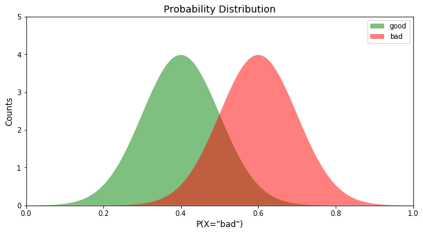
First off, let us assume that our hypothetical model produced some probabilities for predicting the class of each record. As with most binary fraud models, let’s assume our classes are ‘good’ and ‘bad’ and the model produced probabilities of P(X=’bad’). To create this, probability distribution, we plot a Gaussian distribution with different mean values for each class. For more information on Gaussian distribution, read this blog.

import numpy as np
import matplotlib.pyplot as plt
def pdf(x, std, mean):
    cons = 1.0 / np.sqrt(2*np.pi*(std**2))
    pdf_normal_dist = const*np.exp(-((x-mean)**2)/(2.0*(std**2)))
    return pdf_normal_dist
x = np.linspace(0, 1, num=100)
good_pdf = pdf(x,0.1,0.4)
bad_pdf = pdf(x,0.1,0.6)

Now that we have the distribution, let’s create a function to plot the distributions.

def plot_pdf(good_pdf, bad_pdf, ax):
    ax.fill(x, good_pdf, "g", alpha=0.5)
    ax.fill(x, bad_pdf,"r", alpha=0.5)
    ax.set_xlim([0,1])
    ax.set_ylim([0,5])
    ax.set_title("Probability Distribution", fontsize=14)
    ax.set_ylabel('Counts', fontsize=12)
    ax.set_xlabel('P(X="bad")', fontsize=12)
    ax.legend(["good","bad"])

Now let’s use this plot_pdf function to generate the plot:

fig, ax = plt.subplots(1,1, figsize=(10,5))
plot_pdf(good, bad, ax)

Now we have the probability distribution of the binary classes, we can now use this distribution to derive the ROC curve.

Deriving ROC Curve

 
To derive the ROC curve from the probability distribution, we need to calculate the True Positive Rate (TPR) and False Positive Rate (FPR). For a simple example, let’s assume the threshold is at P(X=’bad’)=0.6 .

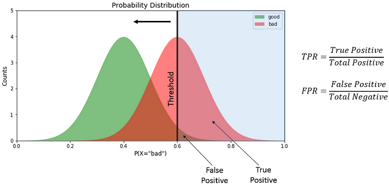
True positive is the area designated as “bad” on the right side of the threshold. False positive denotes the area designated as “good” on the right of the threshold. Total positive is the total area under the “bad” curve while total negative is the total area under the “good” curve. We divide the value as shown in the diagram to derive TPR and FPR. We derive the TPR and FPR different threshold values to get the ROC curve. Using this knowledge, we create the ROC plot function:

def plot_roc(good_pdf, bad_pdf, ax):
    #Total
    total_bad = np.sum(bad_pdf)
    total_good = np.sum(good_pdf)
    #Cumulative sum
    cum_TP = 0
    cum_FP = 0
    #TPR and FPR list initialization
    TPR_list=[]
    FPR_list=[]
    #Iteratre through all values of x
    for i in range(len(x)):
        #We are only interested in non-zero values of bad
        if bad_pdf[i]>0:
            cum_TP+=bad_pdf[len(x)-1-i]
            cum_FP+=good_pdf[len(x)-1-i]
        FPR=cum_FP/total_good
        TPR=cum_TP/total_bad
        TPR_list.append(TPR)
        FPR_list.append(FPR)
    #Calculating AUC, taking the 100 timesteps into account
    auc=np.sum(TPR_list)/100
    #Plotting final ROC curve
    ax.plot(FPR_list, TPR_list)
    ax.plot(x,x, "--")
    ax.set_xlim([0,1])
    ax.set_ylim([0,1])
    ax.set_title("ROC Curve", fontsize=14)
    ax.set_ylabel('TPR', fontsize=12)
    ax.set_xlabel('FPR', fontsize=12)
    ax.grid()
    ax.legend(["AUC=%.3f"%auc])

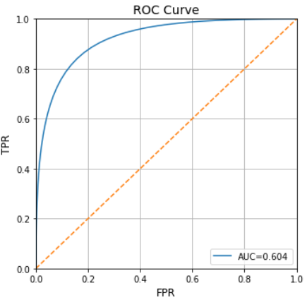
Now let’s use this plot_roc function to generate the plot:

fig, ax = plt.subplots(1,1, figsize=(10,5))
plot_roc(good_pdf, bad_pdf, ax)

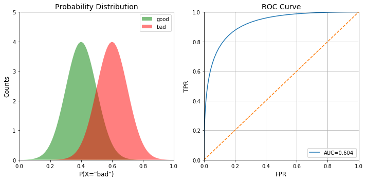
Now plotting the probability distribution and the ROC next to eachother for visual comparison:

fig, ax = plt.subplots(1,2, figsize=(10,5))
plot_pdf(good_pdf, bad_pdf, ax[0])
plot_roc(good_pdf, bad_pdf, ax[1])
plt.tight_layout()

Effect of Class Separation

 
Now that we can derive both plots, let’s see how the ROC curve changes as the class separation (i.e. the model performance) improves. We do this by altering the mean value of the Gaussian in the probability distributions.

x = np.linspace(0, 1, num=100)
fig, ax = plt.subplots(3,2, figsize=(10,12))
means_tuples = [(0.5,0.5),(0.4,0.6),(0.3,0.7)]
i=0
for good_mean, bad_mean in means_tuples:
    good_pdf = pdf(x,0.1,good_mean)
    bad_pdf = pdf(x,0.1,bad_mean)
    plot_pdf(good_pdf, bad_pdf, ax[i,0])
    plot_roc(good_pdf, bad_pdf, ax[i,1])
    i+=1
plt.tight_layout()

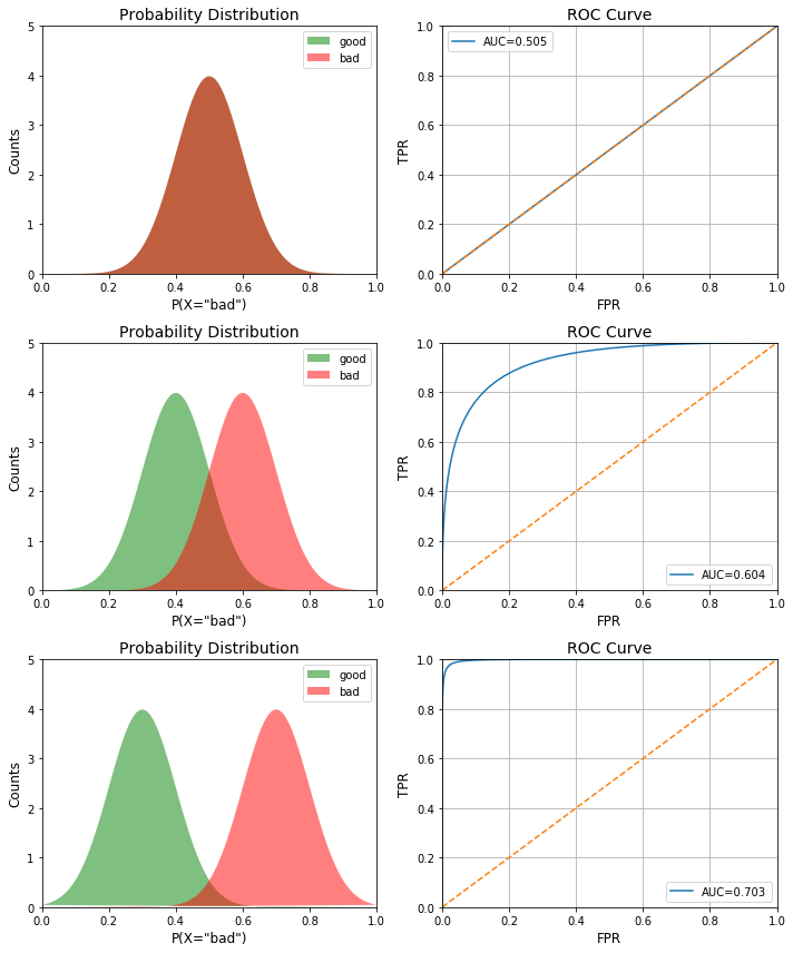
As you can see, the AUC increases as we increase the separation between the classes.

Looking Beyond The AUC

 
Beyond AUC, the ROC curve can also help debug a model. By looking at the shape of the ROC curve, we can evaluate what the model is misclassifying. For example, if the bottom left corner of the curve is closer to the random line, it implies that the model is misclassifying at X=0. Whereas, if it is random on the top right, it implies the errors are occurring at X=1. Also, if there are spikes on the curve (as opposed to being smooth), it implies the model is not stable.

 
Additional Information

• Data Science Interview Guide - Data Science is quite a large and diverse field. As a result, it is really difficult to be a jack of all trades...
• Fraud Detection Under Extreme Class Imbalance - A popular field in data science is fraud analytics. This might include credit/debit card fraud, anti-money laundering...

 
Bio: Syed Sadat Nazrul is using Machine Learning to catch cyber and financial criminals by day... and writing cool blogs by night.

Original. Reposted with permission.

Related:

• Learning Curves for Machine Learning
• Choosing the Right Metric for Evaluating Machine Learning Models – Part 1
• Choosing the Right Metric for Evaluating Machine Learning Models — Part 2