fast.ai Deep Learning Part 1 Complete Course Notes

By Hiromi Suenaga, fast.ai Student

Editor's note: This is one of a series of posts which act as a collection of a set of fantastic notes on the fast.ai machine learning and deep learning learning streams that are freely available online. The author of all of these notes, Hiromi Suenaga -- which, in sum, are a great supplement review material for the course or a standalone resource in their own right -- wanted to ensure that sufficient credit was given to course creators Jeremy Howard and Rachel Thomas in these summaries.

Below you will find links to the posts in this particular series, along with an excerpt from each post. Find more of Hiromi's notes here.

 
My personal notes from machine learning class. These notes will continue to be updated and improved as I continue to review the course to “really” understand it. Much appreciation to Jeremy and Rachel who gave me this opportunity to learn.

 
Deep Learning 2: Part 1 Lesson 1

Underlying function that deep learning uses is called the neural network:

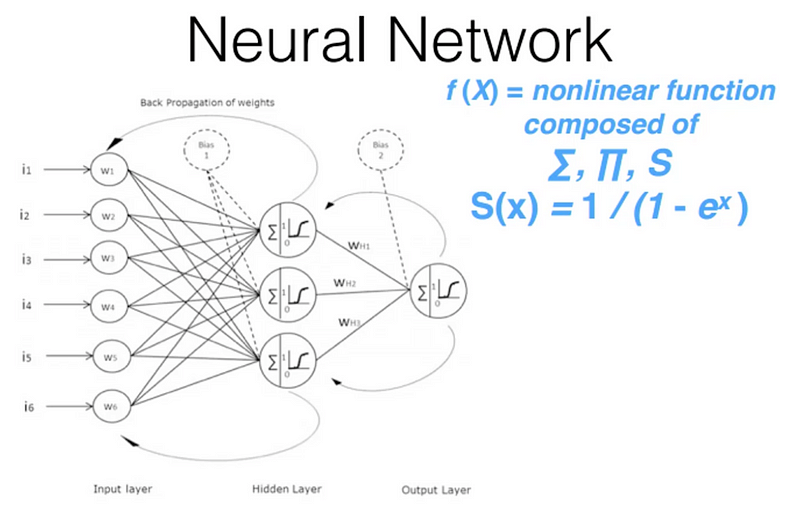
All you need to know for now is that it consists of a number of simple linear layers interspersed with a number of simple non-linear layers. When you intersperse these layers, you get something called the universal approximation theorem. What universal approximation theorem says is that this kind of function can solve any given problem to arbitrarily close accuracy as long as you add enough parameters.

 
Deep Learning 2: Part 1 Lesson 2

• If the learning rate is too small, it will take very long time to get to the bottom
• If the learning rate is too big, it could get oscillate away from the bottom.
• Learning rate finder (learn.lr_find) will increase the learning rate after each mini-batch. Eventually, the learning rate is too high that loss will get worse. We then look at the plot of learning rate against loss, and determine the lowest point and go back by one magnitude and choose that as a learning rate (1e-2 in the example below).
• Mini-batch is a set of few images we look at each time so that we are using the parallel processing power of the GPU effectively (generally 64 or 128 images at a time)

 
Deep Learning 2: Part 1 Lesson 3

We have gotten as far as fully connected layer (it does classic matrix product). In the excel sheet, there is one activation. If we want to look at which one of ten digit the input is, we actually want to calculate 10 numbers.

Let’s look at an example where we are trying to predict whether a picture is a cat, a dog, or a plane, or fish, or a building. Our goal is:

1. Take output from the fully connected layer (no ReLU so there may be negatives)
2. Calculate 5 numbers where each of them is between 0 and 1 and they add up to 1.

To do this, we need a different kind of activation function (a function applied to an activation).

Why do we need non-lineality? If you stack multiple linear layers, it is still just a linear layer. By adding non-linear layers, we can fit arbitrarily complex shapes. The non-linear activation function we used was ReLU.

 
Deep Learning 2: Part 1 Lesson 4

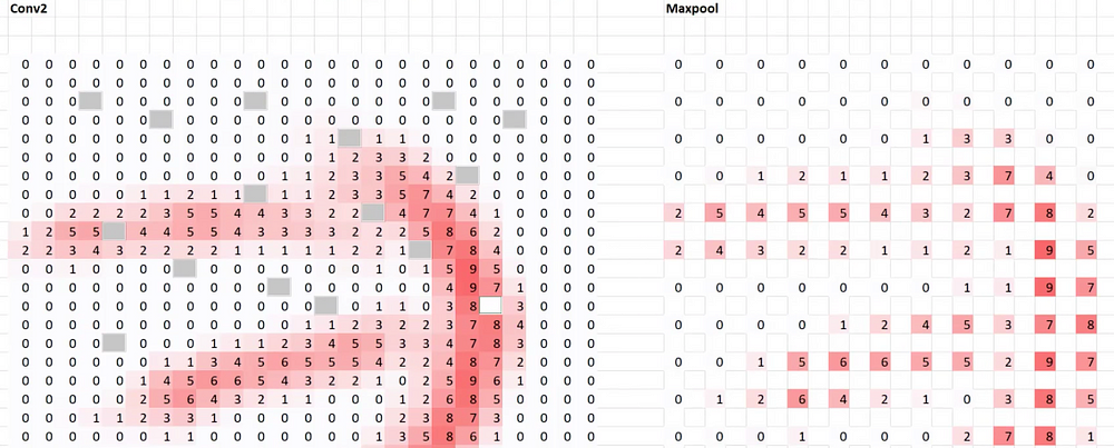
If we applied dropout with p=0.5 to Conv2 layer, it would look like the above. We go through, pick an activation, and delete it with 50% chance. So p=0.5 is the probability of deleting that cell. Output does not actually change by very much, just a little bit.

Randomly throwing away half of the activations in a layer has an interesting effect. An important thing to note is for each mini-batch, we throw away a different random half of activations in that layer. It forces it to not overfit. In other words, when a particular activation that learned just that exact dog or exact cat gets dropped out, the model has to try and find a representation that continues to work even as random half of the activations get thrown away every time.

This has been absolutely critical in making modern deep learning work and just about solve the problem of generalization. Geoffrey Hinton and his colleagues came up with this idea loosely inspired by the way the brain works.

 
Deep Learning 2: Part 1 Lesson 5

When there are much more parameters than data points, regularizations become important. We had seen dropout previously, and weight decay is another type of regularization. Weight decay (L2 regularization) penalizes large weights by adding squared weights (times weight decay multiplier) to the loss. Now the loss function wants to keep the weights small because increasing the weights will increase the loss; hence only doing so when the loss improves by more than the penalty.

The problem is that since we added the squared weights to the loss function, this affects the moving average of gradients and the moving average of the squared gradients for Adam. This result in decreasing the amount of weight decay when there is high variance in gradients, and increasing the amount of weight decay when there is little variation. In other words, “penalize large weights unless gradients varies a lot” which is not what we intended. AdamW removed the weight decay out of the loss function, and added it directly when updating the weights.

 
Deep Learning 2: Part 1 Lesson 6

The second paper to talk about categorical embeddings. FIG. 1. caption should sound familiar as they talk about how entity embedding layers are equivalent to one-hot encoding followed by a matrix multiplication.

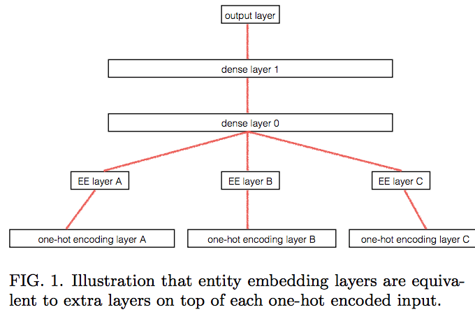
The interesting thing they did was, they took the entity embeddings trained by a neural network, replaced each categorical variable with the learned entity embeddings, then fed that into Gradient Boosting Machine (GBM), Random Forest (RF), and KNN — which reduced the error to something almost as good as neural network (NN). This is a great way to give the power of neural net within your organization without forcing others to learn deep learning because they can continue to use what they currently use and use the embeddings as input. GBM and RF train much faster than NN.

 
Deep Learning 2: Part 1 Lesson 7

Question: How do we choose the size of bptt? There are a couple things to think about:

• the first is that mini-batch matrix has a size of bs (# of chunks) by bptt so your GPU RAM must be able to fit that by your embedding matrix. So if you get CUDA out of memory error, you need reduce one of these.
• If your training is unstable (e.g. your loss is shooting off to NaN suddenly), then you could try decreasing your bptt because you have less layers to gradient explode through.
• If it is too slow [22:44], try decreasing your bptt because it will do one of those steps at a time. for loop cannot be parallelized (for the current version). There is a recent thing called QRNN (Quasi-Recurrent Neural Network) which does parallelize it and we hope to cover in part 2.
• So pick the highest number that satisfies all these.

 
Bio: Hiromi Suenaga is a fast.ai student.

Related:

• An Introduction to Deep Learning for Tabular Data
• Quick Feature Engineering with Dates Using fast.ai
• An Overview of 3 Popular Courses on Deep Learning