Support Vector Machine (SVM) Tutorial: Learning SVMs From Examples

By Abhishek Ghose, 24/7, Inc.

After the Statsbot team published the post about time series anomaly detection, many readers asked us to tell them about the Support Vector Machines approach. It’s time to catch up and introduce you to SVM without hard math and share useful libraries and resources to get you started.

If you have used machine learning to perform classification, you might have heard about Support Vector Machines (SVM). Introduced a little more than 50 years ago, they have evolved over time and have also been adapted to various other problems like regression, outlier analysis, and ranking.

SVMs are a favorite tool in the arsenal of many machine learning practitioners. At [24]7, we too use them to solve a variety of problems.

In this post, we will try to gain a high-level understanding of how SVMs work. I’ll focus on developing intuition rather than rigor. What that essentially means is we will skip as much of the math as possible and develop a strong intuition of the working principle.

 

The Problem of Classification

 
Say there is a machine learning (ML) course offered at your university. The course instructors have observed that students get the most out of it if they are good at Math or Stats. Over time, they have recorded the scores of the enrolled students in these subjects. Also, for each of these students, they have a label depicting their performance in the ML course: “Good” or “Bad.”

Now they want to determine the relationship between Math and Stats scores and the performance in the ML course. Perhaps, based on what they find, they want to specify a prerequisite for enrolling in the course.

How would they go about it? Let’s start with representing the data they have. We could draw a two-dimensional plot, where one axis represents scores in Math, while the other represents scores in Stats. A student with certain scores is shown as a point on the graph.

The color of the point — green or red — represents how he did on the ML course: “Good” or “Bad” respectively.

This is what such a plot might look like:

When a student requests enrollment, our instructors would ask her to supply her Math and Stats scores. Based on the data they already have, they would make an informed guess about her performance in the ML course.

What we essentially want is some kind of an “algorithm,” to which you feed in the “score tuple” of the form (math_score, stats_score). It tells you whether the student is a red or green point on the plot (red/green is alternatively known as a class or label). And of course, this algorithm embodies, in some manner, the patterns present in the data we already have, also known as the training data.

In this case, finding a line that passes between the red and green clusters, and then determining which side of this line a score tuple lies on, is a good algorithm. We take a side — the green side or the red side — as being a good indicator of her most likely performance in the course.

The line here is our separating boundary (because it separates out the labels)or classifier (we use it classify points). The figure shows two possible classifiers for our problem.

 

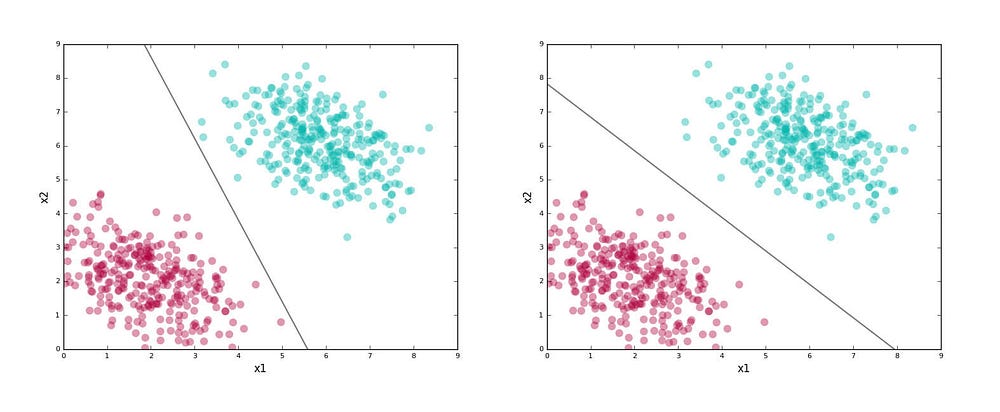
Good vs Bad Classifiers

 
Here’s an interesting question: both lines above separate the red and green clusters. Is there a good reason to choose one over another?

Remember that the worth of a classifier is not in how well it separates the training data. We eventually want it to classify yet-unseen data points (known as test data). Given that, we want to choose a line that captures the general pattern in the training data, so there is a good chance it does well on the test data.

The first line above seems a bit “skewed.” Near its lower half it seems to run too close to the red cluster, and in its upper half it runs too close to the green cluster. Sure, it separates the training data perfectly, but if it sees a test point that’s a little farther out from the clusters, there is a good chance it would get the label wrong.

The second line doesn’t have this problem. For example, look at the test points shown as squares and the labels assigned by the classifiers in the figure below.

The second line stays as far away as possible from both the clusters while getting the training data separation right. By being right in the middle of the two clusters, it is less “risky,” gives the data distributions for each class some wiggle room so to speak, and thus generalizes well on test data.

SVMs try to find the second kind of line. We selected the better classifier visually, but we need to define the underlying philosophy a bit more precisely to apply it in the general case. Here’s a simplified version of what SVMs do:

1. Find lines that correctly classify the training data
2. Among all such lines, pick the one that has the greatest distance to the points closest to it.

The closest points that identify this line are known as support vectors. And the region they define around the line is known as the margin.

Here’s the second line shown with the support vectors: points with black edges (there are two of them) and the margin (the shaded region).

Support Vector Machines give you a way to pick between many possible classifiers in a way that guarantees a higher chance of correctly labeling your test data. Pretty neat, right?

While the above plot shows a line and data in two dimensions, it must be noted that SVMs work in any number of dimensions; and in these dimensions, they find the analogue of the two-dimensional line.

For example, in three dimensions they find a plane (we will see an example of this shortly), and in higher dimensions they find a hyperplane — a generalization of the two-dimensional line and three-dimensional plane to an arbitrary number of dimensions.

Data that can be separated by a line (or in general, a hyperplane) is known as linearly separable data. The hyperplane acts as a linear classifier.

 

Allowing for Errors

 
We looked at the easy case of perfectly linearly separable data in the last section. Real-world data is, however, typically messy. You will almost always have a few instances that a linear classifier can’t get right.

Here’s an example of such data:

Clearly, if we are using a linear classifier, we are never going to be able to perfectly separate the labels. We also don’t want to discard the linear classifier altogether because it does seem like a good fit for the problem except for a few errant points.

How do SVMs deal with this? They allow you to specify how many errors you are willing to accept.

You can provide a parameter called “C” to your SVM; this allows you to dictate the tradeoff between:

1. Having a wide margin.
2. Correctly classifying training data. A higher value of C implies you want lesser errors on the training data.

It bears repeating that this is a tradeoff. You get better classification of training data at the expense of a wide margin.

The following plots show how the classifier and the margin vary as we increase the value of C (support vectors not shown):

Note how the line “tilts” as we increase the value of C. At high values, it tries to accommodate the labels of most of the red points present at the bottom right of the plots. This is probably not what we want for test data. The first plot with C=0.01 seems to capture the general trend better, although it suffers from a lower accuracy on the training data compared to higher values for C.

And since this is a trade-off, note how the width of the margin shrinks as we increase the value of C.

In the previous example, the margin was a “no man’s land” for points. Here, we see it’s not possible anymore to have both a good separating boundary and an associated point-free margin. Some points creep into the margin.

An important practical problem is to decide on a good value of C. Since real-world data is almost never cleanly separable, this need comes up often. We typically use a technique like cross-validation to pick a good value for C.